Data Structures and Program Design Using C++ E-Book

Mercury Learning and Information

• Herausgeber: Packt Publishing
• Kategorie: Fachliteratur
• Sprache: Englisch

Seitenzahl: 477

Veröffentlichungsjahr: 2024

Beschreibung

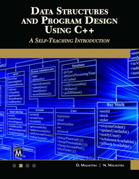
This book introduces the fundamentals of data structures using C++ in a self-teaching format. It covers managing large amounts of information, SEO, and creating Internet/Web indexing services. Practical analogies with real-world applications help explain technical concepts. The book includes end-of-chapter exercises such as programming tasks, theoretical questions, and multiple-choice quizzes.
The course starts with an introduction to data structures and the C++ language, progressing through arrays, linked lists, queues, searching and sorting, stacks, trees, multi-way search trees, hashing, files, and graphs. Each chapter builds on the previous one, ensuring a comprehensive understanding of data structures.
Understanding these concepts is crucial for managing large databases and optimizing web services. This book guides readers from basic to advanced data structure techniques, blending theoretical knowledge with practical skills. Companion files with source code and data sets enhance the learning experience, making this book an essential resource for mastering data structures with C++.

Leseprobe

DATA STRUCTURES AND PROGRAM DESIGN USING C++

A Self-Teaching Introduction

Dheeraj Malhotra

Neha Malhotra

MERCURY LEARNING AND INFORMATION

Dulles, VirginiaBoston, MassachusettsNew Delhi

Copyright © 2019 by MERCURY LEARNING AND INFORMATION LLC.All rights reserved.

This publication, portions of it, or any accompanying software may not be reproduced in any way, stored in a retrieval system of any type, or transmitted by any means, media, electronic display or mechanical display, including, but not limited to, photocopy, recording, Internet postings, or scanning, without prior permission in writing from the publisher.

Publisher: David PallaiMERCURY LEARNING AND INFORMATION22841 Quicksilver DriveDulles, VA [email protected][phone]

D. Malhotra and N. Malhotra. Data Structures and Program Design Using C++.ISBN: 978-1-68392-370-1

The publisher recognizes and respects all marks used by companies, manufacturers, and developers as a means to distinguish their products. All brand names and product names mentioned in this book are trademarks or service marks of their respective companies. Any omission or misuse (of any kind) of service marks or trademarks, etc. is not an attempt to infringe on the property of others.

Library of Congress Control Number: 2018913035

181920321         Printed on acid-free paper in the United States of America.

Our titles are available for adoption, license, or bulk purchase by institutions, corporations, etc. For additional information, please contact the Customer Service Dept. at [phone](toll free). Digital versions of our titles are available at: www.authorcloudware.com and other electronic vendors.

The sole obligation of MERCURY LEARNING AND INFORMATION to the purchaser is to replace the book and/or disc, based on defective materials or faulty workmanship, but not based on the operation or functionality of the product.

Dedicated to ourloving parents and beloved students.

CONTENTS

Preface

Acknowledgments

1 Introduction to Data Structures

1.1Introduction

1.2Types of Data Structures

1.2.1Linear and Non-linear Data Structures

1.2.2Static and Dynamic Data Structures

1.2.3Homogeneous and Non-homogeneous Data Structures

1.2.4Primitive and Non-Primitive Data Structures

1.2.5Arrays

1.2.6Queues

1.2.7Stacks

1.2.8Linked List

1.2.9Trees

1.2.10Graphs

1.3Operations on Data Structures

1.4Algorithms

1.4.1Developing an Algorithm

1.5Approaches for Designing an Algorithm

1.6Analyzing an Algorithm

1.6.1Time-Space Trade-off

1.7Abstract Data Types

1.8Big O Notation

1.9Summary

1.10Exercises

1.11Multiple Choice Questions

2 Introduction to the C++ Language

2.1Introduction

2.2C++ and Its Characteristics

2.3Features of Object-Oriented Programming

2.4Character Set Used in C++

2.5C++ Tokens

2.6Data Types in C++

2.7Structure of a C++ Program

2.7.1Structure of a C++ Program without Classes

2.7.2Structure of a C++ Program with Classes

2.8Operators in C++

2.9Decision Control Statements in C++

2.10Looping Statements in C++

2.11Break and Continue Statements

2.12Functions in C++

2.12.1Passing Arguments to Functions

2.13Structures in C++

2.14Reference Variables in C++

2.15Pointers

2.16Arrays and Pointers

2.17Summary

2.18Exercises

2.18.1Theory Questions

2.18.2Programming Questions

2.18.3Multiple Choice Questions

3 Arrays

3.1Introduction

3.2Definition of an Array

3.3Array Declaration

3.4Array Initialization

3.5Calculating the Address of Array Elements

3.6Operations on Arrays

3.72-D Arrays/ Two-Dimensional Arrays

3.8Declaration of Two-Dimensional Arrays

3.9Operations on 2-D Arrays

3.10Multidimensional Arrays/ N-Dimensional Arrays

3.11Calculating the Address of 3-D Arrays

3.12Arrays and Pointers

3.13Array of Pointers

3.14Arrays and their Applications

3.15Sparse Matrices

3.16Types of Sparse Matrices

3.17Representation of Sparse Matrices

3.18Summary

3.19Exercises

3.19.1Theory Questions

3.19.2Programming Questions

3.19.3Multiple Choice Questions

4 Linked Lists

4.1Introduction

4.2Definition of a Linked List

4.3Memory Allocation in a Linked List

4.4Types of Linked Lists

4.4.1Singly Linked List

4.4.2Operations on a Singly Linked List

4.4.3Circular Linked Lists

4.4.4Operations on a Circular Linked List

4.4.5Doubly Linked List

4.4.6Operations on a Doubly Linked List

4.5Header Linked Lists

4.6Applications of Linked Lists

4.7Polynomial Representation

4.8Summary

4.9Exercises

4.9.1Theory Questions

4.9.2Programming Questions

4.9.3Multiple Choice Questions

5 Queues

5.1Introduction

5.2Definition of a Queue

5.3Implementation of a Queue

5.3.1Implementation of Queues Using Arrays

5.3.2Implementation of Queues Using Linked Lists

5.3.2.1Insertion in Linked Queues

5.3.2.2Deletion in Linked Queues

5.4Operations on Queues

5.4.1Insertion

5.4.2Deletion

5.5Types of Queues

5.5.1Circular Queue

5.5.1.1Limitation of Linear Queues

5.5.1.2Inserting an Element in a Circular Queue

5.5.1.3Deleting an Element from a Circular Queue

5.5.2Priority Queue

5.5.2.1Implementation of a Priority Queue

5.5.2.2Insertion in a Linked Priority Queue

5.5.2.3Deletion in a Linked Priority Queue

5.5.3De-queues (Double-Ended Queues)

5.6Applications of Queues

5.7Summary

5.8Exercises

5.8.1Theory Questions

5.8.2Programming Questions

5.8.3Multiple Choice Questions

6 Searching and Sorting

6.1Introduction to Searching

6.2Linear Search or Sequential Search

6.2.1Drawbacks of a Linear Search

6.3Binary Search

6.3.1Binary Search Algorithm

6.3.2Complexity of a Binary Search Algorithm

6.3.3Drawbacks of a Binary Search

6.4Interpolation Search

6.4.1Working of the Interpolation Search Algorithm

6.4.2Complexity of the Interpolation Search Algorithm

6.5Introduction to Sorting

6.5.1Types of Sorting Methods

6.6External Sorting

6.7Summary

6.8Exercises

6.8.1Theory Questions

6.8.2Programming Questions

6.8.3Multiple Choice Questions

7 Stacks

7.1Introduction

7.2Definition of a Stack

7.3Overflow and Underflow in Stacks

7.4Operations on Stacks

7.5Implementation of Stacks

7.5.1Implementation of Stacks Using Arrays

7.5.2Implementation of Stacks Using Linked Lists

7.5.2.1Push Operation in Linked Stacks

7.5.2.2Pop Operation in Linked Stacks

7.6Applications of Stacks

7.6.1Polish and Reverse Polish Notations and Their Need

7.6.2Conversion from Infix Expression to Postfix Expression

7.6.3Conversion from Infix Expression to Prefix Expression

7.6.4Evaluation of a Postfix Expression

7.6.5Evaluation of a Prefix Expression

7.6.6Parenthesis Balancing

7.7Summary

7.8Exercises

7.8.1Theory Questions

7.8.2Programming Questions

7.8.3Multiple Choice Questions

8 Trees

8.1Introduction

8.2Definitions

8.3Binary Tree

8.3.1Types of Binary Trees

8.3.2Memory Representation of Binary Trees

8.4Binary Search Tree

8.4.1Operations on Binary Search Trees

8.4.2Binary Tree Traversal Methods

8.4.3Creating a Binary Tree Using Traversal Methods

8.5AVL Trees

8.5.1Need of Height-Balanced Trees

8.5.2Operations on an AVL Tree

8.6Summary

8.7Exercises

8.7.1Theory Questions

8.7.2Programming Questions

8.7.3Multiple Choice Questions

9 Multi-Way Search Trees

9.1Introduction

9.2B-Trees

9.3Operations on a B-Tree

9.3.1Insertion in a B-Tree

9.3.2Deletion in a B-Tree

9.4Application of a B-Tree

9.5B+ Trees

9.6Summary

9.7Exercises

9.7.1Review Questions

9.7.2Multiple Choice Questions

10 Hashing

10.1Introduction

10.1.1Difference between Hashing and Direct Addressing

10.1.2Hash Tables

10.1.3Hash Functions

10.1.4Collision

10.1.5Collision Resolution Techniques

10.1.5.1Chaining Method

10.1.5.2Open Addressing Method

10.2Summary

10.3Exercises

10.3.1Review Questions

10.3.2Multiple Choice Questions

11 Files

11.1Introduction

11.2Terminologies

11.3File Operations

11.4File Classification

11.5C vs C++ File Handling

11.6File Organization

11.7Sequence File Organization

11.8Indexed Sequence File Organization

11.9Relative File Organization

11.10Inverted File Organization

11.11Summary

11.12Exercises

11.12.1Review Questions

11.12.2Multiple Choice Questions

12 Graphs

12.1Introduction

12.2Definitions

12.3Graph Representation

12.3.1Adjacency Matrix Representation

12.3.2Adjacency List Representation

12.4Graph Traversal Techniques

12.4.1Breadth First Search

12.4.2Depth First Search

12.5Topological Sort

12.6Minimum Spanning Tree

12.6.1Prim’s Algorithm

12.6.2Kruskal’s Algorithm

12.7Summary

12.8Exercises

12.8.1Theory Questions

12.8.2Programming Questions

12.8.3Multiple Choice Questions

Appendix A

Answers to Selected Exercises

Appendix B

References/ Books/ Webliography

Index

PREFACE

Data structures are the building blocks of computer science. The objective of this text is to emphasize the fundamentals of data structures as an introductory subject. It is designed for beginners who would like to learn the basics of data structures and their implementation using the C++ programming language. With this focus in mind, we present various fundamentals of the subject, well supported with real-world analogies to enable a quick understanding of the technical concepts and to help in identifying appropriate data structures to solve specific, practical problems. This book will serve the purpose of a text/reference book and will be of immense help especially to undergraduate or graduate students of various courses in information technology, engineering, computer applications, and information sciences.

Key Features:

•Practical Applications: Real world analogies as practical applications are given throughout the text to quickly understand and connect the fundamentals of data structures with day to day, real-world scenarios. This approach, in turn, will assist the reader in developing the capability to identify the most appropriate and efficient data structure for solving a specific, real-world problem.

•Frequently Asked Questions: Frequently asked theoretical/practical questions are integrated throughout the content of the book, within related topics to assist readers in grasping the subject.

•Algorithms and Programs: To better understand the fundamentals of data structures at a generic level-followed by its object-oriented implementation in C++, syntax independent algorithms, as well as implemented programs in C++, are discussed throughout the book. This presentation will assist the reader in getting both algorithms and their corresponding implementation within a single book.

•Numerical and Conceptual Exercises: To assist the reader in developing a strong foundation of the subject, various numerical and conceptual problems are included throughout the text.

•Multiple Choice Questions: To assist students for placement-oriented exams in various IT fields, several exercises are suitably chosen and are given in an MCQ format.

Dheeraj MalhotraNeha MalhotraNovember 2018

ACKNOWLEDGMENTS

It is our pleasure to take this opportunity to sincerely thank the people who have extended their kind help and support to us throughout this project.

We are indeed grateful to Chairman VIPS- Dr. S.C. Vats, respected management, faculty and staff members of Vivekananda Institute of Professional Studies (GGS IP University). They are always a source of inspiration for us, and we feel honored because of their faith in us.

We also take this opportunity to extend our gratitude to our mentors Dr. O.P. Rishi (University of Kota), Dr. Jatinder Singh (IKG Punjab Technical University) and Dr. Udyan Ghose (GGS IP University) for their motivation to execute this project.

We are profoundly thankful to Mr. Deepanshu Gupta (VIPS, GGSIPU) for helping us in compiling the codes in this manuscript.

It is not possible to complete a book without the support of a publisher. We are thankful to David Pallai and Jennifer Blaney of Mercury Learning and Information for their enthusiastic involvement throughout the tenure of this project.

Our heartfelt regards to our parents, siblings and family members who cheered us in good times and encouraged us in bad times.

Lastly, we have always felt inspired by our students. Their questioning minds enriched our knowledge, which we have presented in this book.

Dheeraj MalhotraNeha MalhotraNovember 2018

CHAPTER1

INTRODUCTION TO DATA STRUCTURES

In This Chapter

•Introduction

•Types of data structures

•Operations on data structures

•Algorithms

•Approaches for designing an algorithm

•Analyzing an algorithm

•Abstract data types

•Big O notation

•Summary

1.1Introduction

A data structure is an efficient way of storing and organizing the data elements in the computer memory. Data means a value or a collection of values. Structure refers to a method of organizing the data. The mathematical or logical representation of data in the memory is referred as a data structure. The objective of a data structure is to store, retrieve, and update the data efficiently. A data structure can be referred to as elements grouped under one name. The data elements are called members, and they can be of different types. Data structures are used in almost every program and software system. There are various kinds of data structures that are suited for different types of applications. Data structures are the building blocks of a program. For a program to run efficiently, a programmer must choose appropriate data structures. A data structure is a crucial part of data management. As the name suggests, data management is a task which includes different activities like collection of data, organization of data into structures, and much more. Some examples where data structures are used include stacks, queues, arrays, binary trees, linked lists, hash tables, and so forth.

A data structure helps us to understand the relationship of one element to another element and organize it within the memory. It is a mathematical or logical representation or organization of data in memory. Data structures are extensively applied in the following areas:

Compiler Design

Database Management Systems (DBMS)

Artificial Intelligence

Network and Numerical Analysis

Statistical Analysis Packages

Graphics

Operating Systems (OS)

Simulations

As we see in the previous list, there are many applications in which different data structures are used for their operations. Some data structures sacrifice speed for efficient utilization of memory, while others sacrifice memory utilization and result in faster speed. In today’s world programmers aim not just to build a program, but instead to build an effective program. As previously discussed, for a program to be efficient, a programmer must choose appropriate data structures. Hence, data structures are classified into various types. Now, let us discuss and learn about different types of data structures.

Frequently Asked Questions

Q1. Define the term data structure.

Answer.

A data structure is an organization of data in a computer’s memory or disk storage. In other words, a logical or mathematical model of a particular organization of data is called a data structure. A data structure in computer science is also a way of storing data in a computer so that it can be used efficiently. An appropriate data structure allows a variety of important operations to be performed using both resources, that is, memory space and execution time, efficiently.

1.2Types of Data Structures

Data structures are classified into various types.

1.2.1Linear and Non-Linear Data Structures

A linear data structure is one in which the data elements are stored in a linear, or sequential, order; that is, data is stored in consecutive memory locations. A linear data structure can be represented in two ways; either it is represented by a linear relationship between various elements utilizing consecutive memory locations as in the case of arrays, or it may be represented by a linear relationship between the elements utilizing links from one element to another as in the case of linked lists. Examples of linear data structures include arrays, linked lists, stacks, queues, and so on.

A non-linear data structure is one in which the data is not stored in any sequential order or consecutive memory locations. The data elements in this structure are represented by a hierarchical order. Examples of non-linear data structures include graphs, trees, and so forth.

1.2.2Static and Dynamic Data Structures

A static data structure is a collection of data in memory which is fixed in size and cannot be changed during runtime. The memory size must be known in advance, as the memory cannot be reallocated later in a program. One example is an array.

A dynamic data structure is a collection of data in which memory can be reallocated during execution of a program. The programmer can add or remove elements according to his/her need. Examples include linked lists, graphs, trees, and so on.

1.2.3Homogeneous and Non-Homogeneous Data Structures

A homogeneous data structure is one that contains data elements of the same type, for example, arrays.

A non-homogeneous data structure contains data elements of different types, for example, structures.

1.2.4Primitive and Non-Primitive Data Structures

Primitive data structures are the fundamental data structures or predefined data structures which are supported by a programming language. Examples of primitive data structure types are short, integer, long, float, double, char, pointers, and so forth.

Non-primitive data structures are comparatively more complicated data structures that are created using primitive data structures. Examples of non-primitive data structures are arrays, files, linked lists, stacks, queues, and so on.

Classification of different data structures is shown in Figure 1.1.

FIGURE 1.1 Classification of different data structures.

We know that C++ supports various data structures. So, we will now introduce all these data structures, and they will be discussed in detail in the upcoming chapters

Frequently Asked Questions

Q2. Write the difference between primitive data structures and non-primitive data structures.

Answer.

Primitive data structures – The data structures that are typically directly operated upon by machine-level instructions, that is, the fundamental data types such as int, float, char, and so on, are known as primitive data structures.

Non-primitive data structures – The data structures which are not fundamental are called non-primitive data structures.

Frequently Asked Questions

Q3. Explain the difference between linear and non-linear data structures.

Answer.

The main difference between linear and non-linear data structures lies in the way in which data elements are organized. In the linear data structure, elements are organized sequentially, and therefore they are easy to implement in a computer’s memory. In non-linear data structures, a data element can be attached to several other data elements to represent specific relationships existing among them.

1.2.5Arrays

An array is a collection of homogeneous (similar) types of data elements in contiguous memory. An array is a linear data structure because all elements of an array are stored in linear order. The various elements of the array are referenced by their index value, also known as the subscript. In C++, an array is declared using the following syntax:

Syntax – <Data type> array name [size];

The elements are stored in the array as shown in Figure 1.2.

FIGURE 1.2 Memory representation of an array.

Arrays are used for storing a large amount of data of similar type. They have various advantages and limitations.

Advantages of using arrays

1.Elements are stored in adjacent memory locations; hence, searching is very fast, as any element can be easily accessed.

2.Arrays do not support dynamic memory allocation, so all the memory management is done by the compiler.

Limitations of using arrays

1.Insertion and deletion of elements in arrays is complicated and very time-consuming, as it requires the shifting of elements.

2.Arrays are static; hence, the size must be known in advance.

3.Elements in the array are stored in consecutive memory locations which may or may not be available.

1.2.6Queues

A queue is a linear collection of data elements in which the element inserted first will be the element that is taken out first; that is, a queue is a FIFO (First In First Out) data structure. A queue is a popular linear data structure in which the first element is inserted from one end called the REAR end (also called the tail end), and the deletion of the element takes place from the other end called the FRONT end (also called the head).

Practical Application:

For a simple illustration of a queue, there is a line of people standing at the bus stop and waiting for the bus. Therefore, the first person standing in the line will get into the bus first.

In a computer’s memory queues can be implemented using arrays or linked lists. Figure 1.3 shows the array implementation of a queue. Every queue has FRONT and REAR variables which point to the positions where deletion and insertion are done respectively.

FIGURE 1.3 Memory representation of a queue.

1.2.7Stacks

A stack is a linear collection of data elements in which insertion and deletion take place only at the top of the stack. A stack is a Last In First Out (LIFO) data structure, because the last element pushed onto the stack will be the first element to be deleted from the stack. Three operations can be performed on the stack, which include PUSH, POP, and PEEP operations. The PUSH operation inputs an element into the top of the stack, while the POP operation removes an element from the stack. The PEEP operation returns the value of the topmost element in the stack without deleting it from the stack. Every stack has a variable TOP which is associated with it. The TOP pointer stores the address of the topmost element in the stack. The TOP is the position where insertion and deletion take place.

Practical Application:

A real-life example of a stack is if there is a pile of plates arranged on a table. A person will pick up the first plate from the top of the stack.

In a computer’s memory stacks can be implemented using arrays or linked lists. Figure 1.4 shows the array implementation of a stack.

FIGURE 1.4 Memory representation of a stack.

1.2.8Linked List

The major drawback of the array is that the size or the number of elements must be known in advance. Thus, this drawback gave rise to the new concept of a linked list. A linked list is a linear collection of data elements. These data elements are called nodes, which point to the next node using pointers. A linked list is a sequence of nodes in which each node contains one or more than one data field and a pointer which points to the next node. Also, linked lists are dynamic; that is, memory is allocated as and when required.

FIGURE 1.5 Memory representation of a linked list.

In the previous figure we have made a linked list in which each node is divided into two slots:

1.The first slot contains the information/data.

2.The second slot contains the address of the next node.

Practical Application:

A simple real-life example is a train; here each coach is connected to its previous and next coach (except the first and last coach).

The address part of the last node stores a special value called NULL, which denotes the end of the linked list. The advantage of a linked list over arrays is that now it is easier to insert and delete data elements, as we don’t have to do shifting each time. Yet searching for an element has become difficult. Also, more time is required to search for an element, and it also requires high memory space. Hence, linked lists are used where a collection of data elements is required but the number of data elements in the collection is not known to us in advance.

Frequently Asked Questions

Q4. Define the term linked list.

Answer.

A linked list or one-way list is a linear collection of data elements called nodes, where pointers give the linear order. It is a popular dynamic data structure. The nodes in the linked list are not stored in consecutive memory locations. For every data item in a node of the linked list, there is an associated pointer that gives the address location of the next node in the linked list.

1.2.9Trees

A tree is a popular non-linear data structure in which the data elements or the nodes are represented in a hierarchical order. Here, one of the nodes is shown as the root node of the tree, and the remaining nodes are partitioned into two disjointed sets such that each set is a part of a subtree. A tree makes the searching process very easy, and its recursive programming makes a program optimized and easy to understand.

For example, consider a binary tree where R is the root node of the tree. LEFT and RIGHT are the left and right subtrees of R respectively. Node A is designated as the root node of the tree. Nodes B and C are the left and right child of A respectively. Nodes B, D, E, and G constitute the left subtree of the root. Similarly, nodes C, F, H, and I constitute the right subtree of the root.

FIGURE 1.6 A binary tree.

Advantages of a tree

1.The searching process is very fast in trees.

2.Insertion and deletion of the elements have become easier as compared to other data structures.

Frequently Asked Questions

Q5. Define the term binary tree.

Answer.

A binary tree is a hierchical data structure in which each node has at most two children, that is, a left and right child. In a binary tree, the degree of each node can be at most two. Binary trees are used to implement binary search trees, which are used for efficient searching and sorting. A variation of BST is an AVL tree where height of left and right sub tree differs by one . A binary tree is a popular subtype of a k-ary tree, where k is 2.

1.2.10Graphs

Practical Application:

A real-life example of a graph can be seen in workstations where several computers are joined to one another via network connections.

For example, consider a graph G with six vertices and eight edges. Here, Q and Z are neighbors of P. Similarly, R and T are neighbors of S.

FIGURE 1.7 A graph.

1.3Operations on Data Structures

Here we will discuss various operations which are performed on data structures.

•Creation – It is the process of creating a data structure. Declaration and initialization of the data structure are done here. It is the first operation.

•Insertion – It is the process of adding new data elements in the data structure, for example, to add the details of an employee who has recently joined an organization.

•Deletion – It is the process of removing a particular data element from the given collection of data elements, for example, to remove the name of an employee who has left the company.

•Updating – It is the process of modifying the data elements of a data structure. For example, if the address of a student is changed, then it should be updated.

•Searching – It is used to find the location of a particular data element or all the data elements with the help of a given key, for example, to find the names of people who live in New York.

•Sorting – It is the process of arranging the data elements in some order, that is, either ascending or descending order. An example is arranging the names of students of a class in alphabetical order.

•Merging – It is the process of combining the data elements of two different lists to form a single list of data elements.

•Traversal – It is the process of accessing each data element exactly once so that it can be processed. An example is to print the names of all the students of a class.

•Destruction – It is the process of deleting the entire data structure. It is the last operation in the data structure.

1.4Algorithms

An algorithm is a systematic set of instructions combined to solve a complex problem. It is a step-by-finite-step sequence of instructions, each of which has a clear meaning and can be executed in a minimum amount of effort in finite time. In general, an algorithm is a blueprint for writing a program to solve the problem. Once we have a blueprint of the solution, we can easily implement it in any high-level language like C, C++, and so forth. It solves the problem into the finite number of steps. An algorithm written in a programming language is known as a program. A computer is a machine with no brain or intelligence. Therefore, the computer must be instructed to perform a given task in unambiguous steps. Hence, a programmer must define his problem in the form of an algorithm written in English. Thus, such an algorithm should have following features:

1.An algorithm should be simple and concise.

2.It should be efficient and effective.

3.It should be free of ambiguity; that is, the logic must be clear.

Similarly, an algorithm must have following characteristics:

•Input – It reads the data of the given problem.

•Output – The desired result must be produced.

•Process/Definiteness – Each step or instruction must be unambiguous.

•Effectiveness – Each step should be accurate and concise. The desired result should be produced within a finite time.

•Finiteness – The number of steps should be finite.

1.4.1Developing an Algorithm

To develop an algorithm, some steps are suggested:

1.Defining or understanding the problem.

2.Identifying the result or output of the problem.

3.Identifying the inputs required by the problem and choosing the best input.

4.Designing the logic from the given inputs to get the desired output.

5.Testing the algorithm for different inputs.

6.Repeating the previous steps until it produces the desired result for all the inputs.

1.5Approaches for Designing an Algorithm

A complicated algorithm is divided into smaller units which are called modules. Then these modules are further divided into sub-modules. Thus, in this way, a complex algorithm can easily be solved. The process of dividing an algorithm into modules is called modularization. There are two popular approaches for designing an algorithm:

•Top-Down Approach

•Bottom-Up Approach

Now let us understand both approaches.

1.Top-Down Approach – A top-down approach states that the complex/complicated problem/algorithm should be divided into a smaller number of one or more modules. These smaller modules are further divided into one or more sub-modules. This process of decomposition is repeated until we achieve the desired output of module complexity. A top-down approach starts from the topmost module, and the modules are incremented accordingly until a level is reached where we don’t require any more sub-modules, that is, the desired level of complexity is achieved.

FIGURE 1.8 Top-down approach.

2.Bottom-Up Approach – A bottom-up algorithm design approach is the opposite of a top-down approach. In this kind of approach, we first start with designing the basic modules and proceed further toward designing the high-level modules. The sub-modules are grouped together to form a module of a higher level. Similarly, all high-level modules are grouped to form more high-level modules. Thus, this process of combining the sub-modules is repeated until we obtain the desired output of the algorithm.

FIGURE 1.9 Bottom-up approach.

1.6Analyzing an Algorithm

An algorithm can be analyzed by two factors, that is, space and time. We aim to develop an algorithm that makes the best use of both these resources. Analyzing an algorithm measures the efficiency of the algorithm. The efficiency of the algorithm is measured in terms of speed and time complexity. The complexity of an algorithm is a function that measures the space and time used by an algorithm in terms of input size.

Time Complexity – The time complexity of an algorithm is the amount of time taken by an algorithm to run the program completely. It is the running time of the program. The time complexity of an algorithm depends upon the input size. The time complexity is commonly represented by using big O notation. For example, the time complexity of a linear search is O(n).

Space Complexity – The space complexity of an algorithm is the amount of memory space required to run the program completely. The space complexity of an algorithm depends upon the input size.

Time Complexity is categorized into three types:

1.Best Case Running Time – The performance of the algorithm will be best under optimal conditions. For example, the best case for a binary search occurs when the desired element is the middle element of the list. Another example can be of sorting; that is, if the elements are already sorted in a list, then the algorithm will execute in best time.

2.Average Case Running Time – It denotes the behavior of an algorithm when the input is randomly drawn from a given collection or distribution. It is an estimate of the running time for “average” input. It is usually assumed that all inputs of a given size are likely to occur with equal probability.

3.Worst Case Running Time – The behavior of the algorithm in this case concerns the worst possible case of input instance. The worst case running time of an algorithm is an upper bound on the running time for any input. For example, the worst case for a linear search occurs when the desired element is the last element in the list or the element does not exist in the list.

Frequently Asked Questions

Q6. Define the time complexity.

Answer.

Time complexity is a measure which evaluates the count of the operations performed by a given algorithm as a function of the size of the input. It is the approximation of the number of steps necessary to execute an algorithm. It is commonly represented with asymptotic notation, that is, O(g) notation, also known as big O notation, where g is the function of the size of the input data.

1.6.1Time-Space Trade-Off

In computer science, time-space trade-off is a way of solving a particular problem either in less time and more memory space or in more time and less memory space. But if we talk in practical terms, designing such an algorithm in which we can save both space and time is a challenging task. So, we can use more than one algorithm to solve a problem. One may require less time, and the other may require less memory space to execute. Therefore, we sacrifice one thing for the other. Hence, there exists a time-space or time-memory trade-off between algorithms. Thus, this time-space trade-off gives the programmer a rational choice from an informed point of view. So, if time is a big concern for a programmer, then he or she might choose a program which takes less or the minimum time to execute. On the other hand, if space is a prime concern for a programmer, then, in that case, he or she might choose a program that takes less memory space to execute at the cost of more time.

1.7Abstract Data Types

An abstract data type (ADT) is a popular mathematical model of the data objects which define a data type along with various functions that operate on these objects. To understand the meaning of an abstract data type, we will simply break the term into two parts, that is, “data type” and “abstract.” The data type of a variable is a collection of values which a variable can take. There are various data types in C++ that include integer, float, character, long, double, and so on. When we talk about the term “abstract” in the context of data structures, it means apart from detailed specification. It can be considered as a description of the data in a structure with a list of operations to be executed on the data within the structure. Thus, an abstract data type is the specification of a data type that specifies the mathematical and logical model of the data type. For example, when we use stacks and queues, then at that point of time our prime concern is only with the data type and the operations to be performed on those structures. We are not worried about how the data will be stored in the memory. Also, we don’t bother about how push() and pop() operations work. We just know that we have two functions available to us, so we have to use them for insertion and deletion operations.

1.8Big O Notation

The performance of an algorithm, that is, time and space requirements, can be easily compared with other competitive algorithms using asymptotic notations such as the big O notation, the Omega notation, and the Theta notation. The algorithmic complexity can be easily approximated using asymptotic notations by simply ignoring the implementation-dependent factors. For instance, we can compare various available sorting algorithms using big O notation or any other asymptotic notation.

An algorithm with O(1) complexity is referred to as a constant computing time algorithm. Similarly, an algorithm with O(n) complexity is referred to as a linear algorithm, O(n2) for quadratic algorithms, O(2n) for exponential time algorithms, O(nk) for polynomial time algorithms, and O (log n) for logarithmic time algorithms.

An algorithm with complexity of the order of O(log2n) is considered as one of the best algorithms, while an algorithm with complexity of the order of O(2n) is considered as the worst algorithm. The complexity of computations or the number of iterations required in various types of functions may be compared as follows:

O(log2n) < O(n) < O (n log2n) < O(n2)<O(n3) < O(2n)

1.9Summary

•A data structure determines a way of storing and organizing the data elements in the computer memory. Data means a value or a collection of values. Structure refers to a way of organizing the data. The mathematical or logical representation of data in the memory is referred as a data structure.

•Data structures are classified into various types which include linear and non-linear data structures, primitive and non-primitive data structures, static and dynamic data structures, and homogeneous and non-homogeneous data structures.

•A linear data structure is one in which the data elements are stored in a linear or sequential order; that is, data is stored in consecutive memory locations. A non-linear data structure is one in which the data is not stored in any sequential order or consecutive memory locations.

•A static data structure is a collection of data in memory which is fixed in size and cannot be changed during runtime. A dynamic data structure is a collection of data in which memory can be reallocated during execution of a program.

•Primitive data structures are fundamental data structures or predefined data structures which are supported by a programming language. Non-primitive data structures are comparatively more complicated data structures that are created using primitive data structures.

•A homogeneous data structure is one that contains all data elements of the same type. A non-homogeneous data structure contains data elements of different types.

•An array is a collection of homogeneous (similar) types of data elements in contiguous memory.

•A queue is a linear collection of data elements in which the element inserted first will be the element taken out first, that is, a FIFO data structure. A queue is a linear data structure in which the first element is inserted from one end called the REAR end and the deletion of the element takes place from the other end called the FRONT end.

•A linked list is a sequence of nodes in which each node contains one or more than one data field and a pointer which points to the next node.

•A stack is a linear collection of data elements in which insertion and deletion take place only at one end called the TOP of the stack. A stack is a Last In First Out (LIFO) data structure, because the last element added to the top of the stack will be the first element to be deleted from the top of the stack.

•A tree is a non-linear data structure in which the data elements or the nodes are represented in a hierarchical order. Here, an initial node is designated as the root node of the tree, and the remaining nodes are partitioned into two disjointed sets such that each set is a part of a subtree.

•A binary tree is the simplest form of a tree. A binary tree consists of a root node and two subtrees known as the left subtree and right subtree, where both the subtrees are also binary trees.

•A graph is a general tree with no parent-child relationship. It is a non-linear data structure which consists of vertices or nodes and the edges which connect those vertices with one another.

•An algorithm is a systematic set of instructions combined to solve a complex problem. It is a step-by-finite-step sequence of instructions, each of which has a clear meaning and can be executed in a minimum amount of effort in finite time.

•The process of dividing an algorithm into modules is called modularization.

•The time complexity of an algorithm is described as the amount of time taken by an algorithm to run the program completely. It is the running time of the program.

•The space complexity of an algorithm is the amount of memory space required to run the program completely.

•An ADT (Abstract Data Type) is a mathematical model of the data objects which define a data type as well as the functions to operate on these objects.

•Big O notation is one of the most popular analysis characterization schemes, since it provides an upper bound on the complexity of an algorithm.

1.10Exercises

1.What do you understand by a good program?

2.Explain the classification of data structures.

3.What is an algorithm? Discuss the characteristics of an algorithm.

4.What are the various operations that can be performed on the data structures? Explain each of them with an example.

5.Differentiate an array with a linked list.

6.Explain the terms time complexity and space complexity.

7.What do you understand by the complexity of an algorithm?

8.Write a short note on graphs.

9.What is the process of modularization?

10.Differentiate between stacks and queues with examples.

11.What is meant by abstract data types (ADT)? Explain in detail.

12.Discuss the worst case, best case, and average case time complexity of an algorithm.

13.Write a brief note on trees.

14.Explain how you can develop an algorithm to solve a complex problem.

15.Explain time-memory trade-off in detail.

1.11Multiple Choice Questions

1.Which of the following data structures is a FIFO data structure?

a.Array

b.Stacks

c.Queues

d.Linked List

2.How many maximum children can a binary tree have?

a.0

b.2

c.1

d.3

3.Which of the following data structures uses dynamic memory allocation?

a.Graphs

b.Linked Lists

c.Trees

d.All of these

4.In a queue, deletion is always done from the ______

a.Front end

b.Rear end

c.Middle

d.None of these

5.Which data structure is used to represent complex relationships between the nodes?

a.Linked Lists

b.Trees

c.Stacks

d.Graphs

6.Which of the following is an example of a heterogeneous data structure?

a.Array

b.Structure

c.Linked list

d.None of these

7.In a stack, insertion and deletion takes place from the ______

a.Bottom

b.Middle

c.Top

d.All of these

8.Which of the following is not part of the Abstract Data Type (ADT) description?

a.Operations

b.Data

c.Both (a) and (b)

d.None of the above

9.Which of the following data structures allows deletion at both ends of the list but insertion at one end only?

a.Stack

b.Input Restricted Dequeue

c.Output Restricted Dequeue

d.Priority Queue

10.Which of the following data structures is a linear type?

a.Trees

b.Graphs

c.Queues

d.None of the above

11.Which one of the following is beneficial when the data is stored and has to be retrieved in reverse order?

a.Stack

b.Linked List

c.Queue

d.All of the above

12.A binary search tree whose left and right subtree differ in height by 1 at most is a ____

a.Red Black Tree

b.M way search tree

c.AVL Tree

d.None of the above

13.The operation of processing each element in the list is called ________

a.Traversal

b.Merging

c.Inserting

d.Sorting

14.Which of the following are the two primary measures of the efficiency of an algorithm?

a.Data & Time

b.Data & Space

c.Time & Space

d.Time & Complexity

15.Which one of the following cases does not exist/occur in complexity theory?

a.Average Case

b.Worst Case

c.Best Case

d.Minimal Case

CHAPTER 2

INTRODUCTION TO THE C++ LANGUAGE

In This Chapter

•Introduction

•C++ and Its Characteristics

•Features of Object-Oriented Programming

•Character Set Used in C++

•C++ Tokens

•Data Types in C++

•Structure of a C++ Program

•Operators in C++

•Decision Control Statements in C++

•Looping Statements in C++

•Break and Continue Statements

•Functions in C++

•Structures in C++

•Reference Variables in C++

•Pointers

•Arrays and Pointers

•Summary

•Exercises

2.1Introduction

A programming language like C++ is a set of commands that are specifically designed for instructing the computer devices to perform specific tasks. There are three levels of programming languages, which are commonly known as high-level, middle-level, and low-level languages. The level determines the degree of closeness of the programming language with the hardware. Generally, high-level languages are portable, which means they can operate in different machines with fewer modifications. A high-level language, instead of being machine-dependent, is oriented toward problem-solving, whereas a low-level language is limited by the characteristics of the hardware. Each programming language is chosen to solve a particular class of problems depending upon the type of program. However, the C++ language is a middle-level language that directly interacts with the hardware with almost no limitations and can abstract lower layers, and thus it can work as one of the powerful high level-languages.

2.2C++ and Its Characteristics

The C++ language was created and developed by Bjarne Stroustrup, a Danish computer scientist at Bell Labs, in New Jersey in 1979. The C++ language supports all the features, flexibilities, and attributes of C language. It also introduces various new features that were designed to support object-oriented programming. C++ was initially known with the new name of “C with Classes.” Thus, C++ is the object-oriented version of C. When creating C++, Stroustrup successfully accomplished his goal of retaining the efficiency, flexibility, and philosophy of C while also adding new features for OOP (Object Oriented Programming). The following characteristics distinguish C++ from other programming languages:

•C++ is object-oriented programming that allows the program to interact with the help of the objects. It allows greater usability of code in a productive way.

•C++ is portable; that is, the code written in C++ can be compiled in any of the computer systems without any modifications.

•Codes written in C++ are short in comparison with other languages.

•C++ is compatible with the C language; that is, any code written in C can easily be included in C++ with little or no modifications, but the reverse is not possible.

2.3Features of Object-Oriented Programming

The following are the various features or characteristics of object-oriented programming:

•Objects – An object is a container in which the data is stored in the combination of variables, functions, and data structures. An object is that component of a program that interacts with the other parts/pieces of the program. They are the fundamental runtime entities of a program.

•Classes – The building block of C++ that leads to object-oriented programming is a class. A class is actually a user-defined data type that holds its own data members and member functions. It is a way to bind the data members and its functions together. A class can be accessed by creating an object of that class. When a class is defined, we can create any number of objects as an instance of the class. Thus, a class is a collection of objects of similar types. Classes provide a convenient method for packing together a group of logically related data items and functions that work on them. The classes are declared by using the keyword “class” with the following syntax:

class class_name { access specifier: //can be public, private or protected data members ; ------------ ------------ member functions() { ------------ ------------ } };

Where class_name is the name of the class, data members are the variables to be used, and the member functions are the methods to access the data members.

Frequently Asked Questions

Q1. What is the difference between the base and derived class?

Answer.

When creating a class, instead of writing completely new data members and member functions, the programmer can designate that the new class should inherit the members of an existing class. This existing class is known as a base class, and the new class is known as a derived class. A class can be derived from more than one class, which means it can inherit data and functions from multiple base classes.

•Encapsulation – Encapsulation is a process of wrapping up of data members and member functions into a single unit. It is the mechanism which keeps the code and the data safe from external interference. It implies that there is no direct access granted to the data; that is, it is hidden. So, in order to access that data, we must interact with the object that is responsible for the data. This is also known as data hiding. The process of encapsulation makes the data of the system more secure and reliable.

Practical Application:

The most common example of encapsulation is a capsule. In a capsule, all the medicines are encapsulated inside a single capsule.

•Inheritance – Inheritance is the process of deriving a new class from the existing one. The existing class is known as the “base class” or “parent class” or “superclass.” The new class is known as the “derived class” or “child class” or “subclass.” The process of inheritance allows the child classes to inherit all the features, that is, variables and methods, of their parent class. Thus, the derived classes will have all the features of their base class, and the programmer can add some new features specific to the derived class. There are five types of inheritances supported in C++, which are as follows:

1.Single Inheritance –A class derived from a single base class is known as single inheritance.

2.Multilevel Inheritance – Classes derived from the already derived classes are known as multilevel inheritance.

3.Multiple Inheritance – A class derived from more than one base class is known as multiple inheritance.

4.Hybrid Inheritance – Hybrid inheritance refers to the combination of one or more types of inheritances.

5.Hierarchical Inheritance – When more than one class is derived from a single base class, it is known as hierarchical inheritance.

Practical Application:

The most common real-life example of inheritance is your family, in which your grandfather is the head of the family (base class/ parent class), your father is the child of the grandfather (derived class/ child class), and you are the child of your father (another derived class).

•Polymorphism – The word polymorphism is derived from the word poly, which means many, and the word morph, which means forms. Therefore, anything that exists in more than one form is referred to as a polymorph. Thus, polymorphism means the ability to make more than one form. Polymorphism usually occurs when there is a hierarchy of classes and the classes are related by inheritance. Polymorphism is considered as one of the most important features of object-oriented programming. Polymorphism is of two types:

1.Compile Time Polymorphism (Static Polymorphism) – It is done using function overloading and operator overloading.

2.Runtime Polymorphism (Dynamic Polymorphism) – It is done using method overriding or virtual functions.

Practical Application:

A person exhibits different roles in different situations; that is, he/she is a child for his/her father, he/she is a student for his/her teachers, he/she is a friend for his/her friends, and so on.

•Abstraction – The process of abstraction is somewhat related to the idea of hiding data that is not essential. Abstraction refers to the act of displaying only the essential features and hiding the background details and explanations that are not needed for the presentation. This is also known as data abstraction. Abstraction is one of the vital features provided by the object-oriented C++ programming language. Since the classes use the concept of data abstraction, they are known as Abstract Data Types (ADT). An abstract data type is a popular mathematical model of the data objects which define a data type along with various functions that operate on these objects. The process of abstraction in C++ is implemented using classes. The class decides which data member will be visible to the outside world and vice versa.

Practical Application:

Consider a man driving a bus. The man only knows that pressing the accelerator will increase the speed of the bus and that applying the brakes decreases the speed of the bus. The man does not know how pressing the accelerator increases the speed or how applying the brakes decreases the speed. Hence, he does not know the inner mechanism of the bus.

Frequently Asked Questions

Q2. Explain the differences between abstraction and encapsulation.

Answer.

Data abstraction refers to providing only essential information to the outside world and hiding the background details, that is, representing the needed information in the program without presenting all the details. On the other hand, encapsulation is an object-oriented programming concept that binds together the data and the functions that manipulate the data and thus keeps them safe from the outside world.

•Message Passing – Message passing is the process of communication between objects. An object-oriented program consists of objects that communicate by sending and receiving information from each other. A message for an object is a request for the execution of a procedure, and thus it will invoke a method in the receiving object that generates the desired results. Message passing involves three things: the name of the object, the name of the function, and the data/information to be sent.

•Dynamic Binding – Dynamic binding is the process by which the code that has to be executed for a given procedure call is known at runtime rather than at the compile time. It is also known as dynamic dispatch. It is an object-oriented programming concept, and it is also related to inheritance and polymorphism.

FIGURE 2.1 Features of object-oriented programming.

Frequently Asked Questions

Q3. Explain how one can achieve data hiding in C++.

Answer.

Encapsulation supports data hiding by making use of three access specifiers of a class.

1.Public – If a class member is declared as public, it can be used anywhere without the class restrictions.

2.Private – If a class member is declared as private, it can be used by the members of the class.

3.Protected – If a class member is declared as protected, it can only be used by the members of the class and the members of the class derived from the class.

2.4Character Set Used in C++

The character set allowed in C++ consists of the following characters:

1.Alphabets – It includes uppercase as well as lowercase letters of English, i.e., {A, B, C... ., Z} and {a, b, c... ., z}.

2.Digits – It includes decimal digits, i.e. {0, 1, 2 . . ., 9}.

3.White Spaces – It includes spaces, enters, and tabs.

4.Special Characters